The Logistic Map is a model for the growth of a single-species population having non-overlapping generations (for instance children are born in the spring and by next spring are mature and productive - some insect populations are examples), and living in an environment having limited resources. "Limited resources" enters the model as a competition term: individuals must compete for available food.
How do we build this model? Let Pn stand for the population in generation n:
P0 is the initial population, the size of the population when we start observng it.
P1 is the population in the first generation after we start observing.
P2 is the population in the second generation after we start observing.
and so on.
We would like to find a relation between Pn and Pn+1. If we find this relation, then knowing the population in any generation we can determine the population in all successive generations. What do we know?
Let's start by ignoring competition. We'll add that effect later. Then what part of the current generation will be present in the next generation? Some will die, so the population decreases by its death rate D. Some will be born, so the population increases by its birth rate B. That is,
Pn+1 = (1 + B - D)*Pn.
This is just Malthus' model, and the future is easy to predict.
If
Now we incorporate the competition effect. First, competition occurs between pairs of animals: two fish trying to catch the same insect, two lions trying to bring down the same wildebeest, two catepillars trying to eat the same blade of grass, two students competing for the only A in the class (just kidding - is anyone still reading this?). If C stands for the competition factor, the population model becomes
Pn+1 = (1 + B - D)*Pn - C*(number of competitive pairs).
So how many competitive pairs are in a population of N animals?
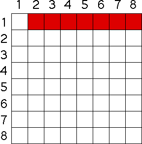
For example, suppose the population consists of eight animals. Animal 1 can compete with animal 2, with animal 3, ..., with animal 8. Assuming no bipolar disorders in the population, animal 1 cannot compete with itself. So there are seven competitive pairs involving animal 1. These are colored red in the chart.
 |
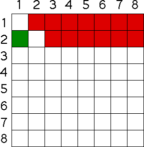
What about animal 2? Certainly, it cannot compete with itself, so as we count up the competitive pairs, we might think there are seven involving animal 2. But we must be a bit more careful. We do not want to count the pairing of animal 2 and animal 1, because we have already accounted for the competiton between animals 1 and 2. So the "animal 2 competing with animal 1" square, colored green in the chart, is not counted. So we have six new competitive pairs: animal 2 with animal 3, animal 2 with animal 4, ..., animal 2 with animal 8.
 |
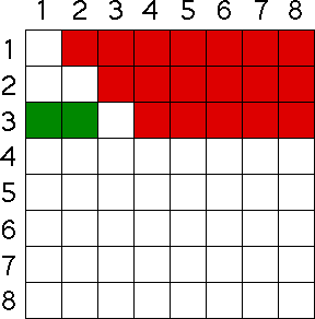
What about animal 3? Certainly, it cannot compete with itself, and we have already counted the competiton between animal 1 and animal 3, and between animal 2 and animal 3, both colored green in the chart. So we are left with five new competitive pairs.
 |
By now the pattern should be clear: the number of competitive
pairs is
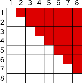 |
In general, for a population of N animals, the number of
competitive pairs is
Pn+1 = (1 + B - D)*Pn - C*(Pn - 1)*Pn/2.
We could use this equation, but our later calculations will be
much simpler if we spend a bit of time recasting the model. Instead of measuring
the actual population number Pn, suppose instead we use the related
variable
xn+1 = (1 + B - D + C/2)*xn*(1 - xn)
This is still too long, so we give the coefficient (1 + B - D + C/2) the name s. Finally, we have the Logistic Map
xn+1 = s*xn*(1 - xn)
the idealized model of a single-species wth limited resources. Robert May's pioneering study of this model, "Simple mathematical models with very complicated dynamics," is one of the main catalysts for the current interest in chaos.
The graph is a parabola opening downward, and passing through
the points
0 <= s <= 4.
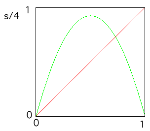 |
As s changes within this range, the orbit x0, x1 = L(x0), x2 = L(x1), ... undergoes a remarkably rich range of behaviors. For more details, see the following demonstration.